(This is part two of my Gnutella exploration series. Please read the Gnutella Explanation article first if you are not already familiar with Gnutella.)

At its peak, Limewire was installed on a third of desktop computers and estimates from the year prior showed a concurrent node count in the millions. It hit this level of adoption while staying decentralized and avoiding the need for a global file index or coordination servers. More importantly, the network still survives today despite minimal upkeep.

Early versions of Gnutella searched the network using a technique called flood routing. Your computer sent a query to its neighbors. Those neighbors sent it to their neighbors. The process continued until the query ran out of hops or reached a machine with a matching file.

Flood routing was beautifully simple, but it created a snowball effect for bandwidth usage. Most of the computers receiving a query had nothing relevant to offer. They still had to accept the message, inspect it, remember it, and forward it onward.

In the previous article, I described Gnutella queries as though they simply flooded across the network. This was true, but I was kinda lying to keep the article short.

Flood routing was OK when Gnutella was an experimental network with a few thousand users. Blindly bothering every reachable computer was no longer viable once the network hit mainstream adoption. Based on my Internet Archive archaeology digs, this practice likely came to an end around the year 2003.

Flood routing is a convenient half-truth we tell for the sake of moving an explanation along, like the time I told my son that semicolons in JavaScript are optional.

Later Gnutella clients (and the ones surviving today) still pass queries through a mesh of peers, but they are much more selective about which peers they decide to bother. They do this without central file indexes and without requiring any participant to reveal an exact list of shared files.

The newer search system was called the Query Routing Protocol, or QRP.

QRP allowed one computer to advertise a compact, approximate summary of the search terms available behind it. A peer could then ask a useful question before forwarding a query: Is there any chance this connection leads to a matching file? The answer is one of two choices: maybe or certainly not.

This system was more complicated than the flood routing system in the first generation of Gnutella clients, but it scaled nicely.

The Old Routing System

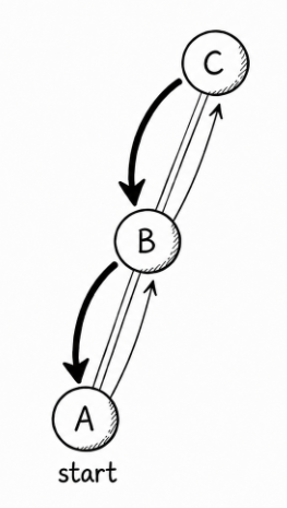
You can't really call it a network protocol if there is only one working implementation. That's just network software, not a protocol. A good protocol should be simple enough that independent developers can implement it, and flood routing met this goal despite efficiency issues.

You can fit the entire query model in your head:

1. Send a query to every connected peer.
2. Decrease its TTL.
3. Have those peers repeat the process until the TTL reaches zero.
4. Suppress duplicate queries using the query's unique identifier.
5. Return any results along remembered reverse routes.

This simplicity gave early Gnutella an ecosystem of diverse clients and, importantly, people actually using the network. Flood routing was not free, though.

Suppose every peer has four connections. The first peer might forward a query to four neighbors. Each of those peers normally excludes the connection from which the query arrived, so a tree-like expansion would start at 4, then expand to 12, 36, 108, and so on.

A real mesh contains cycles, duplicate suppression, and peers with different connection counts, so the actual numbers vary. The important part is that the amount of traffic still grows very quickly.

Most of those peers will not have anything relevant to the search, but they must receive the message, parse it, inspect it, remember its identifier, and decide whether to forward it again.

The network therefore spends most of its query bandwidth proving that peers do not have the requested file.

This is tolerable when the network contains a few thousand machines. It becomes expensive when the network contains millions of machines and every user is typing searches at the same time.

The scalability problems were eventually demonstrated with sciencey PDFs that clearly did the math.

Leaves and Ultrapeers

Early Gnutella was an undifferentiated mesh of peers. Later versions that used QRP divided nodes into two roles:

• A leaf sat at the edge of the network.
• An ultrapeer participated in a highly connected upper tier.

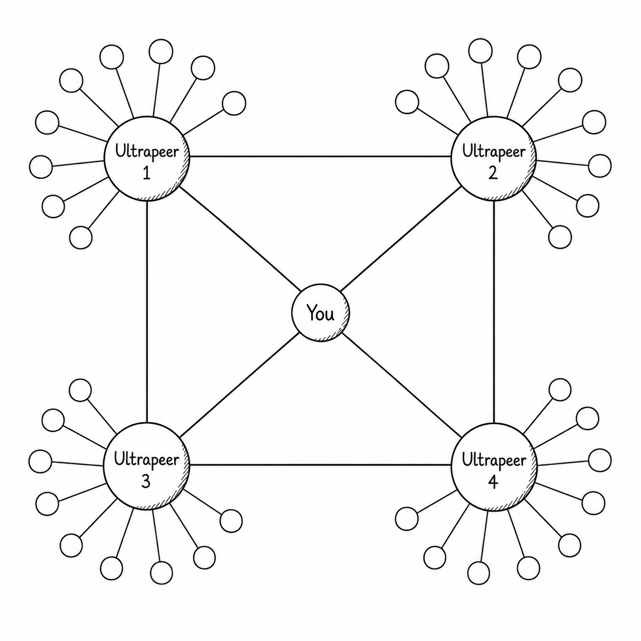
This may sound like client-server architecture, but there was no permanent server and no central authority deciding who could become an ultrapeer.

An ultrapeer was still an ordinary Gnutella user running an ordinary Gnutella client. The difference was that an ultrapeer, unlike a leaf node, had enough bandwidth, uptime, memory, and network reach to perform additional routing work. Ultrapeers were usually those super lucky power users with a DSL connection and a high-end Windows 2000 box with 2 GBs of RAM.

Some clients will automatically promote a node based on things such as uptime, firewall status, available memory, file descriptors, and bandwidth.

A more plebeian peer on a dial-up connection behind a firewall, or with low uptime would operate as a leaf.

Leaves maintained connections to several ultrapeers for redundancy. Ultrapeers maintained connections to other ultrapeers and accepted collections of leaves beneath them.

Why Two Tiers?

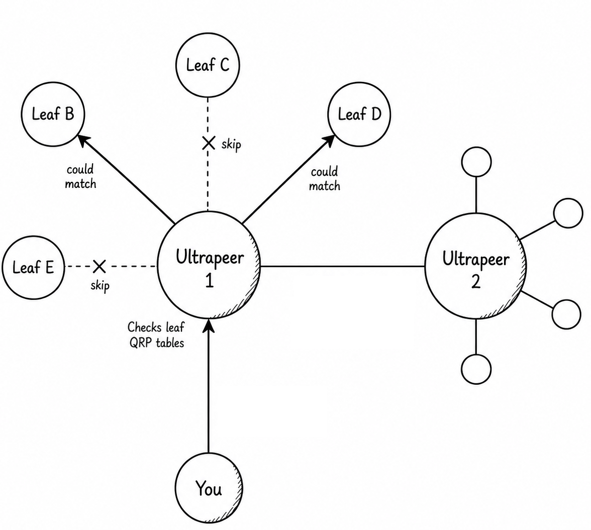
Consider what happens when a leaf sends a query to its ultrapeer.

Under pure flood routing, the ultrapeer would send that query to every other connected leaf, whether or not any of them shared relevant files.

Under QRP, each leaf periodically gives the ultrapeer a compact representation of all the words in its current file library. It's a bit more complicated than just uploading a list of file names. This is called a QRP table, and the ultrapeer holds onto one QRP table per connected leaf.

The underlying data structure allows the ultrapeer to treat the index as a function for determining file availability on a remote node. The function's input is a question: Does leaf X have file Y? The output is Probably yes or Definitely not.

When a query arrives, the ultrapeer checks those tables. For example, if a query arrives for Ubuntu Server 2026 Live CD ISO, the ultrapeer might determine that leaves E and C definitely do not have the file, but leaves B and D might. Therefore, the query is sent to B and D but not C or E.

Using an opaque data structure- a Bloom filter, sort of- the yes/no question is much cheaper to answer than wasting bandwidth by sending the full query to every leaf and waiting for most of them to say nothing.

QRP is primarily applied at the edges of the ultrapeer network. An ultrapeer stores the QRP table received from each leaf separately.

Whenever a keyword query reaches that ultrapeer, it checks the query against each leaf's table. A matching table means the leaf might have a result. A nonmatching table means the query should not be sent.

This check happens whenever an ultrapeer considers forwarding a keyword query to one of its leaves. It is the most direct and important use of QRP.

QRP tables are usually used only for leaf-to-ultrapeer routing. They do not generally create a map of the full network. Some nodes support a thing called last-hop QRP, where the ultrapeer creates a merged summary of all connected leaves to improve ultra-to-ultra query routing, but that is a more complicated matter.

False Positives vs. False Negatives

QRP tables are approximate.

A false positive occurs when the table says a peer connection might match, but no matching file exists. The query travels down one unnecessary connection. Some bandwidth is wasted, but the search still works.

A false negative occurs when the table says a connection cannot match even though a real result exists behind it. The query is discarded, and the user never sees the file.

False positives wastes a little bandwidth, but false negatives hides content.

QRP's table construction is therefore conservative. Its not trying to prove that a connection will produce a result. It makes a best effort guess to route queries to useful endpoints.

Let's take a look at how the tables actually work.

Prerequisite Knowledge: Hash Functions

You can skip this section if you already know what a hash function is.

A hash function accepts some input and deterministically converts it into a number.

Imagine a fictional hash function that produces a number from 0 through 999:

hash("ubuntu") = 412
hash("server") = 731
hash("iso")    = 044

The same input always produces the same output.

Different inputs will usually produce different outputs, but not always. There are more possible words than there are numbers from 0 through 999, so eventually two unrelated words must produce the same number. This is called a collision.

QRP uses this property to turn words into table positions.

The hash does not need to be cryptographically secure. We are not protecting a password or verifying a software download. We only need every compatible Gnutella client to calculate the same table position for the same word.

Prerequisite Knowledge: Bloom Filters, Sort Of

You can also skip this section if you already understand Bloom filters.

A Bloom filter is an extremely compact, approximate representation of a set. Its main operation is asking: Is this item in the set?

A Bloom filter can answer in two ways: Probably and Definitely not.

It cannot reliably answer with 100% certainty because unrelated values may collide and set the same positions.

A QRP table feels very much like a Bloom filter, although it is not exactly the textbook data structure.

The useful mental model is still the same: A QRP table is a lossy, compacted set of search terms.

If a required slot is absent, the connection cannot match that term. If the slot is present, the connection is worth considering.

What Gets Stored in a QRP Table?

Since a QRP table is not a list of files, it does not contain literal filenames or information about the files. It only contains enough information to answer a yes/no question about whether the data exists.

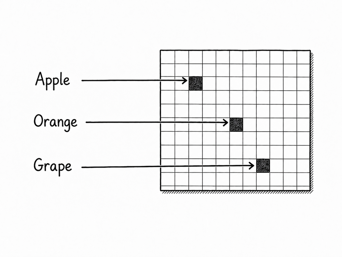
A client starts by canonicalizing the names of its shared files into tokens. This includes operations such as normalizing text- spaces, capitalization, and so on- and separating it into searchable words.

A file named:

Ubuntu Server 2024.iso

might contribute terms resembling:

ubuntu
server
2024
iso

The client does not necessarily insert only complete words.

For example, a long word might contribute forms conceptually resembling:

ubuntu
ubunt
ubun

This allows some prefix searches to find the correct route without inserting every imaginable substring.

Each indexed form is hashed into a table position:

ubuntu  → hash → slot 41,292
server  → hash → slot 17,104
iso     → hash → slot 52,881

The original text is not stored in that slot. The slot only answers the yes/no question, so slots act more like a checklist.

Repeated words are deduplicated during query matching, and terms shorter than three bytes are excluded from the QRP word vector.

I ran an experiment using a real directory containing approximately 6,300 files with filenames of varying lengths. Storing the filenames as plain text required roughly 365 KiB. A QRP table can summarize those filenames in a fraction of that space.

When compacted to one bit per slot, a 65,536-slot table occupies exactly 8 KiB.

Table sizes are selected in powers of two.

A table that is too small becomes crowded. As more terms collide with one another, more positions are marked as present. Eventually, almost every query appears to match, and the table stops saving bandwidth. Peers can respond by constructing a larger table.

How QRP Tables Move Around

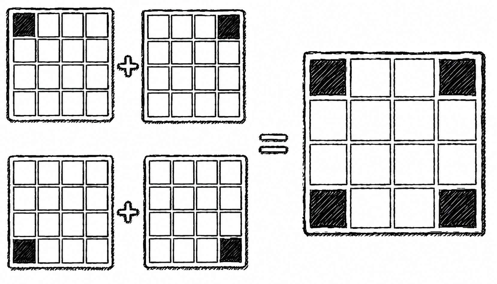
A leaf must send its table to each ultrapeer it connects to.

It would be wasteful to resend a completely unrelated structure every time one file is added or removed, so QRP defines two important message types: RESET and PATCH.

RESET messages instruct a peer to throw away the table currently associated with the sender and prepare a new empty table of a certain size.

The RESET establishes properties such as the number of slots in the new table.

PATCH messages then transform that empty table into the sender's current state.

Unchanged entries are represented as zeros or other no-op values. Because most entries usually do not change, those long runs of zeros compress extremely well over the network.

RESET and PATCH messages are direct-connection messages. They are not flooded across the Gnutella network.

A patch sequence may be split across several messages, but the receiver expects the completed sequence to account for every slot in the logical table.

Matching a Query Against a Table

When a search arrives, the receiving client performs approximately the same canonicalization process used while constructing the table.

A query such as:

Ubuntu Server ISO

becomes a vector of QRP-indexed words.

Each indexed term is hashed into a table slot. The client checks whether those slots are present in the table associated with a connection.

The obvious algorithm would require every word to appear:

ubuntu = present
server = present
iso    = present

If even one word were absent, the query would not be sent down that connection. Most clients apply fuzzy matching that sends the query if a certain threshold is met.

Extra Functionality: Ultra-to-Ultra Queries

I mentioned that QRP tables are used for leaf-to-ultrapeer communication. Sometimes QRP tables can be used for ultra-to-ultra query routing.

An ultrapeer can construct a combined table from its own shared files and the QRP tables supplied by eligible, directly connected leaves.

The ultrapeer may send this combined table to neighboring ultrapeers that advertise support for last-hop QRP.

The combined table indicates that the ultrapeer's own files or one of its directly connected leaves might match these terms. It is important to keep in mind that this does not try to map resources beyond the ultrapeer's directly connected leaves.

Suppose an ultrapeer is considering sending a query to a neighboring ultrapeer.

If the query has more than one hop remaining, the ultrapeer does not use the neighbor's QRP table as a hard filter. The neighbor might forward the query farther into the network, beyond the files represented by its local table.

If the query has exactly one hop remaining, the situation is different.

The neighboring ultrapeer cannot send the query farther through the backbone. All it can do is inspect its own files and forward the query to its leaves.

Those are exactly the resources represented by its combined QRP table.

At that point, a negative QRP match becomes useful, because it is confirmable that nothing available on the final hop can match, so there is no need to send the query there.

QRP therefore can filter leaves connected directly to an ultrapeer and also neighboring ultrapeers when the query is on its final hop.

Conclusion

QRP is a fun but overlooked aspect of late-era Gnutella clients that survived into what is left of the network today. It managed to filter noise effectively at scale without needing the exactness required for a distributed hash table. I am not aware of any extant P2P systems that use QRP tables for content discovery other than Gnutella2.

Not Covered in this Article

There are several implementation details that deserve their own investigation:

• Four-bit and one-bit PATCH negotiation
• Patch compression
• Unicode canonicalization
• SHA-1 and other URN searches
• Handling tables that become excessively dense
• Hops-flow restrictions
• Flow-control behavior for overloaded leaves
• How frequently tables are rebuilt and transmitted
• Compatibility differences between clients
• GUESS, which provides another way to perform targeted Gnutella searches

Further Reading

• Gnutella Explanation - Part one of this series
• Query Routing for the Gnutella Network / mirror - Christopher Rohrs's original QRP proposal
• GTK-Gnutella source code - One of the best surviving records of deployed Gnutella behavior. QRP implementation shown here
• Why Gnutella Can't Scale. No, Really - A critique of the original flood-routing network